Bayesian Updating of Hurricane Vulnerability Functions

Research Question

Can enhanced building vulnerability curves be generated by combining prior knowledge from rapid impact assessments with observed event-based damage data sourced from social media? The project updates vulnerability curves — functions mapping sustained wind speed to expected building damage ratio — using Hurricane Dorian (2019) observations documented on YouTube, then feeds the refined curves into GRADE (Global Rapid post-disaster damage Estimation).

Vulnerability Curves

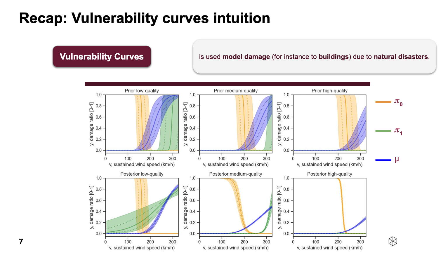
Vulnerability curves model the expected damage to buildings from natural disasters. Each plot contains three curves against sustained wind speed (km/h):

—π₀ (orange) — probability of zero damage
—π₁ (green) — probability of total loss given non-zero damage
—μ (blue) — mean damage ratio

Model — Zero-One Inflated Beta (ZOIB)

The ZOIB distribution handles the three-part nature of damage data: zero damage, partial damage, and total loss. The likelihood function is:

f_ZOIB(y; π₀, π₁, μ, φ) =

π₀ if y = 0

(1 − π₀) · π₁ if y = 1

(1 − π₀)(1 − π₁) · f_beta(y; μ_y, φ) if y ∈ (0, 1)

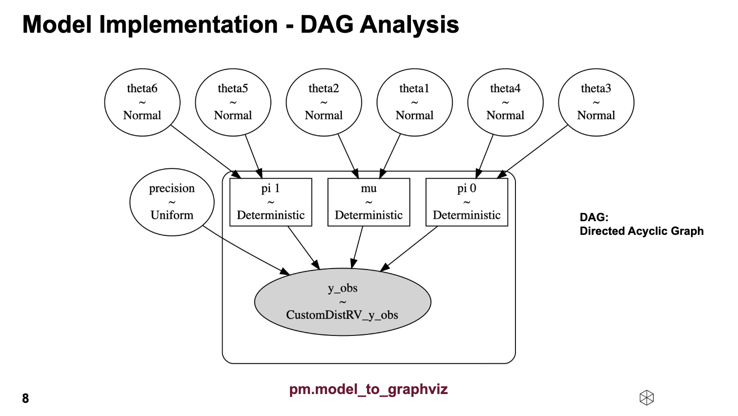
—μ_y = Φ(ln(v / θ₁) / θ₂) — mean damage via cumulative log-normal
—π₀ = logit⁻¹(θ₃ + θ₄ · v) — probability of zero damage
—π₁ = logit⁻¹(θ₅ + θ₆ · v) — probability of total loss

Sampler: NUTS · 3000 samples · tune=1000 · 3 chains.

DAG — Model Structure

Directed Acyclic Graph of the ZOIB model — DAG: 7 stochastic parameters (θ₁–θ₆ ~ Normal, φ ~ Uniform) → 3 deterministic nodes (μ, π₀, π₁) → y_obs (CustomDistRV)

Prior Parameter Settings

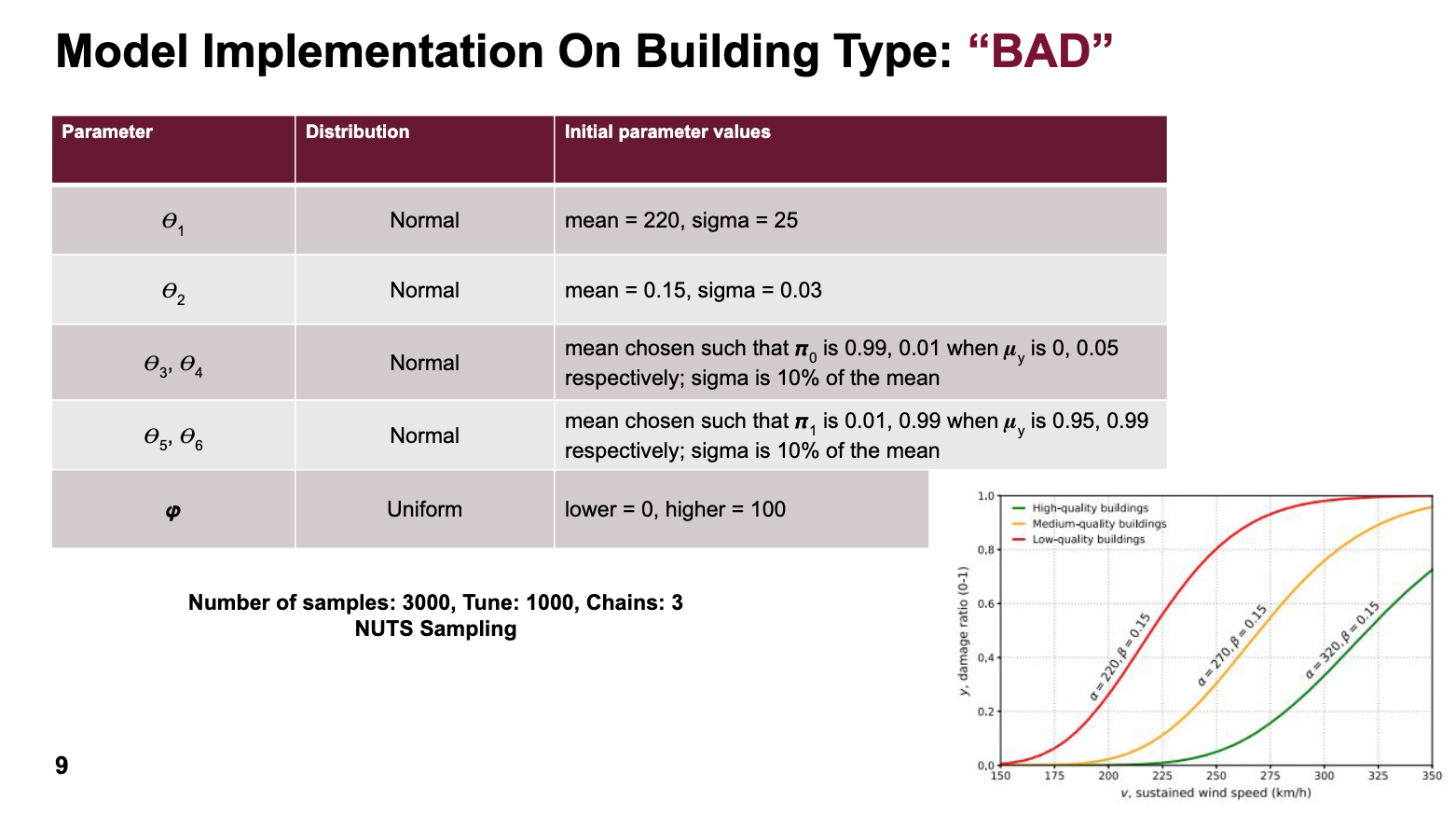
Model implementation parameters for BAD building type — Prior parameter settings for "BAD" (low quality) building type — θ₁ mean=220, θ₂ mean=0.15, φ ~ Uniform(0,100)

Parameter	BAD (low)	MEDIUM	GOOD (high)
θ₁ (alpha)	220	270	320
θ₂ (beta)	0.15	0.15	0.15
φ (precision)	Uniform(0, 40)	Uniform(0, 40)	Uniform(0, 40)

Data — Hurricane Dorian (2019)

—498 YouTube videos screened → 15 relevant videos selected
—3 experts analysed 732 buildings with known geolocations, assigning damage ratios
—Wind field data: max_wind_field.tif — raster of peak sustained wind speeds

Key Findings

—Parameter recovery — posterior means closely match true values (e.g. θ₄ estimated −164.82 vs actual −164.16)
—Convergence fix — bimodal posterior for θ₁ resolved by reducing φ upper bound from 100 → 40
—Low autocorrelation — drops to near zero after lag 1, confirming efficient NUTS sampling
—Discrepancy found — posterior plots matched original authors' generated files, but those files didn't match the published paper — original authors notified

CNN Extension — Satellite Damage Classification

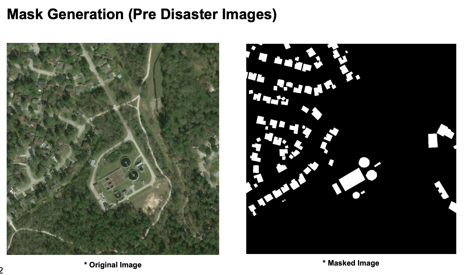
As an original contribution, a CNN pipeline was built using the xBD satellite imagery dataset (Hurricanes Michael, Harvey, Matthew and others) to classify building damage from pre/post-disaster image pairs.

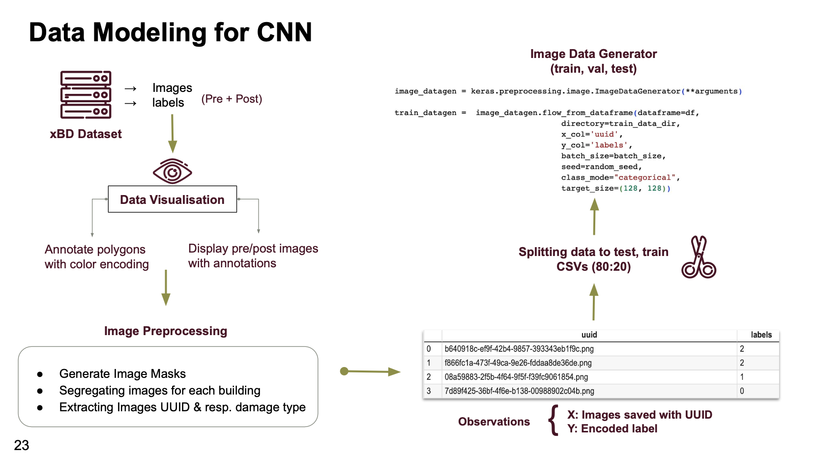
Mask generation from pre-disaster satellite images — Mask generation (pre-disaster) — original aerial image → binary building footprint mask used to isolate individual buildings for classification

CNN data modelling pipeline from xBD dataset — Data pipeline: xBD dataset → polygon annotation with colour-encoded damage labels → image preprocessing → 80/20 train/test CSV split

Level	Label	Description
0	No Damage	No structural, water, or shingle damage
1	Minor Damage	Roof elements missing, visible cracks, partial burning
2	Major Damage	Partial wall/roof collapse, surrounded by water or mud
3	Destroyed	Completely collapsed, scorched, or no longer present

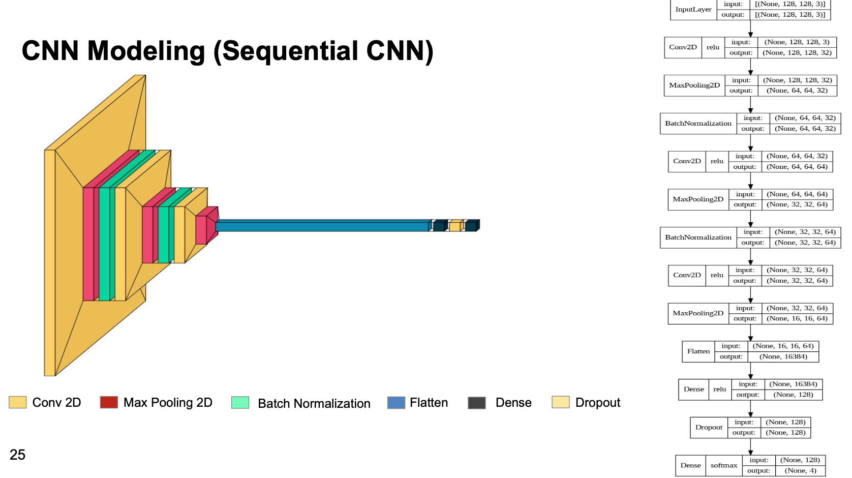
Sequential CNN architecture — Conv2D × 3 + BatchNorm + MaxPooling + Dropout → Flatten → Dense → 4-class softmax (128×128 input)

—Sequential CNN — ~75.7% accuracy, train/val accuracy nearly identical over 30 epochs (minimal overfitting)
—ResNet50 (transfer learning) — custom CNN branch (4096) + ResNet50 (8192) concatenated → Dense → 4-class softmax

Stack

PyMC Bayesian Inference NUTS Sampler ZOIB Distribution CNN ResNet50 TensorFlow / Keras xBD Dataset Python R